Transit access isochrones Agency

Drop a pin and see where a rider can travel on your network within a time budget — combining the walk to a stop, the wait for service, the in-vehicle ride, and the walk from the final stop — drawn as 15 / 30 / 45-minute contours, with the population, jobs, and equity populations reachable inside each.

Where Demographic coverage tells you who lives near your stops, access isochrones tell you where a rider can go from a stop — the temporal, schedule-aware companion to the buffer-based coverage analysis. It's an Agency feature.

What it is

The Access Isochrones panel answers the question no buffer-based tool can: from a given point, what can a rider reach on your network in N minutes? It runs a schedule-based transit router over your in-memory feed and combines three legs of a trip into one reachable area:

• Access — the walk from the origin pin to nearby boardable stops.
• Transit — riding the network: waiting for the next departure, the in-vehicle time, and any transfers, computed from your stop_times (and frequencies.txt) for the chosen service day and departure time.
• Egress — the walk from each reachable stop out to the surrounding streets, drawn as a real routed walkshed.

The union of those reachable areas, clipped to each time budget, is the isochrone. Alongside the map contours, the panel tallies the population, jobs, and equity populations (minority, low-income, zero-vehicle households) inside each contour — the same Census plumbing as the coverage analysis.

When to use it

• Grant narratives and New/Small Starts. "How many jobs can a resident of this low-income tract reach in 45 minutes by transit?" is the standard accessibility framing in FTA filings and regional transportation plans. Access isochrones produce a defensible, documented number.
• Equity analysis with a temporal dimension. Title VI and coverage tell you who lives near service; isochrones tell you what destinations that service actually connects them to.
• Comparing a proposed change. Run the analysis from a key origin on today's network, then again with a proposed route on or off (via route visibility), and compare the residents and jobs reached.
• Siting and outreach. Evaluate transit access from a proposed development, a job center, a hospital, or a neighborhood that's raised a service request.

How to use it in GTFS·X

1. Open the feed in the editor and click Access under Analysis in the left sidebar.
2. Click Set origin on map and click the map to drop the trip origin (drag the pin afterward to move it).
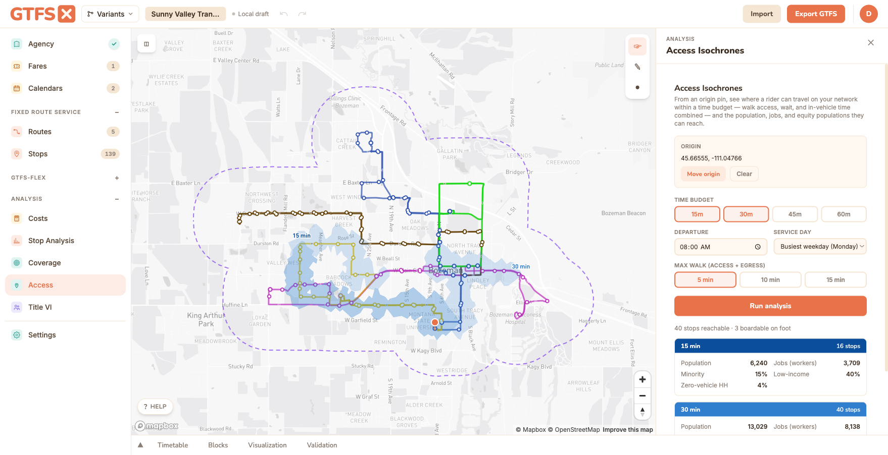
3. Pick your time budgets (15 / 30 / 45 / 60 minutes — choose one or several), a departure time, the service day (defaults to the feed's busiest weekday), and the maximum walk for the access and egress legs.
4. Click Run analysis. GTFS·X routes the network and draws the routed walksheds — because it makes a real walking-isochrone request per reachable stop, a run takes a few seconds (the button shows "Analyzing…").
5. Read the contours on the map (darkest = closest reach, each labeled with its time budget) and the per-budget readout in the sidebar: stops reached, population, jobs, and equity shares.

Methodology

• Routing engine. Reach is computed with RAPTOR (Round-Based Public Transit Routing), the standard algorithm for schedule-based travel-time analysis. It runs entirely in your browser over the feed's stop_times, one round per transfer, returning the earliest arrival time at every stop in the network from the chosen departure time. Frequency-based trips (frequencies.txt) are expanded to synthetic departures, and only the calendars active on the selected service day are considered.
• Access leg. Stops within the walk-time budget of the origin (at an assumed walking speed) seed the router, so the trip clock includes the time it takes to reach the first stop.
• Egress leg — routed walksheds. For each stop reachable within a budget, GTFS·X draws a street-network walkshed (a Mapbox walking isochrone that follows the actual pedestrian network), not a fixed-radius circle, and unions them into the contour. This is the same engine as the Agency-plan network walksheds in the Coverage panel.
• Opportunities. Population, jobs, and equity populations inside each contour are apportioned from US Census ACS block groups overlapping the polygon, through the same summation the coverage analysis uses, so the figures are consistent across the two tools.
• Contours. A single hue with stepped saturation — the closest (shortest-time) band is the most saturated, longer budgets lighter — the standard travel-time-isochrone convention.

Limits

• One departure time. Each run is for a single departure moment, so the result is sensitive to which bus the rider just caught or missed. Run a few departure times to see the range; departure-window averaging is planned.
• Walk legs. The access leg uses a straight-line walk-time to decide which stops are boardable; the egress contour drawn on the map is the real routed walkshed. Neither models elevation, crossing delays, or wait-to-cross.
• Opportunity counts are apportioned. Population, jobs, and equity figures are ACS estimates apportioned to the reachable area; they share the vintage and caveats of the coverage analysis, and ACS block-group data covers the 50 states plus DC.
• Schedule, not real time. Routing uses the published schedule; it does not apply real-time delays, and GTFS-Flex / demand-response zones are not routed.
• Best on small and mid-size feeds. The router runs in the browser; very large feeds are slower, and each reachable stop adds a walking-isochrone request (capped per run).